This documentation is for an unreleased version of Apache Flink. We recommend you use the latest stable version.
Performance Tuning
Performance Tuning #
SQL is the most widely used language for data analytics. Flink’s Table API and SQL enables users to define efficient stream analytics applications in less time and effort. Moreover, Flink Table API and SQL is effectively optimized, it integrates a lot of query optimizations and tuned operator implementations. But not all of the optimizations are enabled by default, so for some workloads, it is possible to improve performance by turning on some options.
In this page, we will introduce some useful optimization options and the internals of streaming aggregation, regular join which will bring great improvement in some cases.
The streaming aggregation optimizations mentioned in this page are all supported for Group Aggregations and Window TVF Aggregations (except Session Window TVF Aggregation) now.
MiniBatch Aggregation #
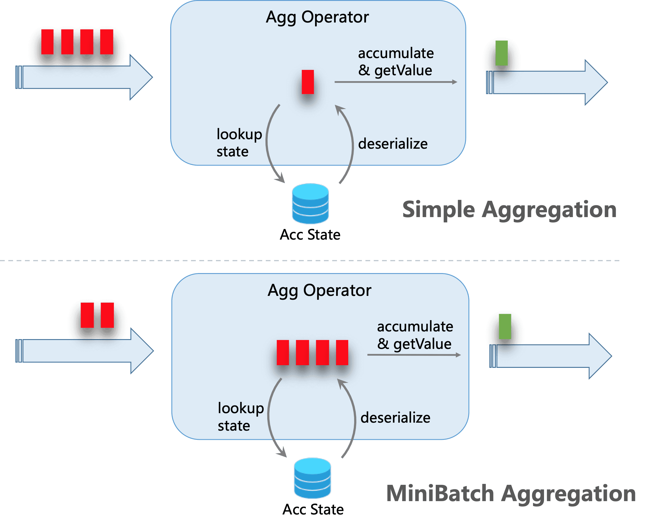
By default, group aggregation operators process input records one by one, i.e., (1) read accumulator from state, (2) accumulate/retract record to the accumulator, (3) write accumulator back to state, (4) the next record will do the process again from (1). This processing pattern may increase the overhead of StateBackend (especially for RocksDB StateBackend). Besides, data skew, which is very common in production, will worsen the problem and make it easy for the jobs to be under backpressure situations.
The core idea of mini-batch aggregation is caching a bundle of inputs in a buffer inside of the aggregation operator. When the bundle of inputs is triggered to process, only one operation per key to access state is needed. This can significantly reduce the state overhead and get a better throughput. However, this may increase some latency because it buffers some records instead of processing them in an instant. This is a trade-off between throughput and latency.
The following figure explains how the mini-batch aggregation reduces state operations.
MiniBatch optimization is disabled by default for group aggregation. In order to enable this optimization, you should set options table.exec.mini-batch.enabled, table.exec.mini-batch.allow-latency and table.exec.mini-batch.size. Please see configuration page for more details.
MiniBatch optimization is always enabled for Window TVF Aggregation, regardless of the above configuration. Window TVF aggregation buffer records in managed memory instead of JVM Heap, so there is no risk of overloading GC or OOM issues.
The following examples show how to enable these options.
// instantiate table environment
TableEnvironment tEnv = ...;

// access flink configuration
TableConfig configuration = tEnv.getConfig();
// set low-level key-value options
configuration.set("table.exec.mini-batch.enabled", "true"); // enable mini-batch optimization
configuration.set("table.exec.mini-batch.allow-latency", "5 s"); // use 5 seconds to buffer input records
configuration.set("table.exec.mini-batch.size", "5000"); // the maximum number of records can be buffered by each aggregate operator task
// instantiate table environment
val tEnv: TableEnvironment = ...

// access flink configuration
val configuration = tEnv.getConfig()
// set low-level key-value options
configuration.set("table.exec.mini-batch.enabled", "true") // enable mini-batch optimization
configuration.set("table.exec.mini-batch.allow-latency", "5 s") // use 5 seconds to buffer input records
configuration.set("table.exec.mini-batch.size", "5000") // the maximum number of records can be buffered by each aggregate operator task
# instantiate table environment
t_env = ...

# access flink configuration
configuration = t_env.get_config()
# set low-level key-value options
configuration.set("table.exec.mini-batch.enabled", "true") # enable mini-batch optimization
configuration.set("table.exec.mini-batch.allow-latency", "5 s") # use 5 seconds to buffer input records
configuration.set("table.exec.mini-batch.size", "5000") # the maximum number of records can be buffered by each aggregate operator task
Local-Global Aggregation #
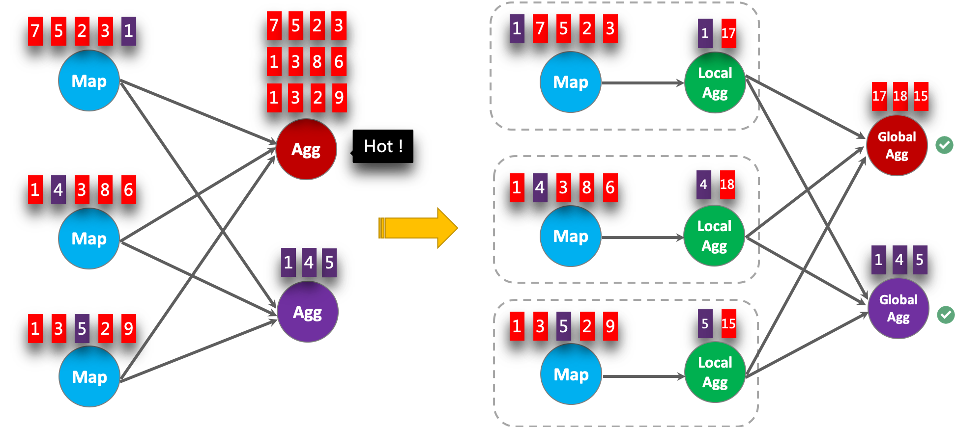
Local-Global is proposed to solve data skew problem by dividing a group aggregation into two stages, that is doing local aggregation in upstream firstly, and followed by global aggregation in downstream, which is similar to Combine + Reduce pattern in MapReduce. For example, considering the following SQL:
SELECT color, sum(id)
FROM T
GROUP BY color
It is possible that the records in the data stream are skewed, thus some instances of aggregation operator have to process much more records than others, which leads to hotspot. The local aggregation can help to accumulate a certain amount of inputs which have the same key into a single accumulator. The global aggregation will only receive the reduced accumulators instead of large number of raw inputs. This can significantly reduce the network shuffle and the cost of state access. The number of inputs accumulated by local aggregation every time is based on mini-batch interval. It means local-global aggregation depends on mini-batch optimization is enabled.
The following figure shows how the local-global aggregation improve performance.
The following examples show how to enable the local-global aggregation.
// instantiate table environment
TableEnvironment tEnv = ...;

// access flink configuration
TableConfig configuration = tEnv.getConfig();
// set low-level key-value options
configuration.set("table.exec.mini-batch.enabled", "true"); // local-global aggregation depends on mini-batch is enabled
configuration.set("table.exec.mini-batch.allow-latency", "5 s");
configuration.set("table.exec.mini-batch.size", "5000");
configuration.set("table.optimizer.agg-phase-strategy", "TWO_PHASE"); // enable two-phase, i.e. local-global aggregation
// instantiate table environment
val tEnv: TableEnvironment = ...

// access flink configuration
val configuration = tEnv.getConfig()
// set low-level key-value options
configuration.set("table.exec.mini-batch.enabled", "true") // local-global aggregation depends on mini-batch is enabled
configuration.set("table.exec.mini-batch.allow-latency", "5 s")
configuration.set("table.exec.mini-batch.size", "5000")
configuration.set("table.optimizer.agg-phase-strategy", "TWO_PHASE") // enable two-phase, i.e. local-global aggregation
# instantiate table environment
t_env = ...

# access flink configuration
configuration = t_env.get_config()
# set low-level key-value options
configuration.set("table.exec.mini-batch.enabled", "true") # local-global aggregation depends on mini-batch is enabled
configuration.set("table.exec.mini-batch.allow-latency", "5 s")
configuration.set("table.exec.mini-batch.size", "5000")
configuration.set("table.optimizer.agg-phase-strategy", "TWO_PHASE") # enable two-phase, i.e. local-global aggregation
Split Distinct Aggregation #
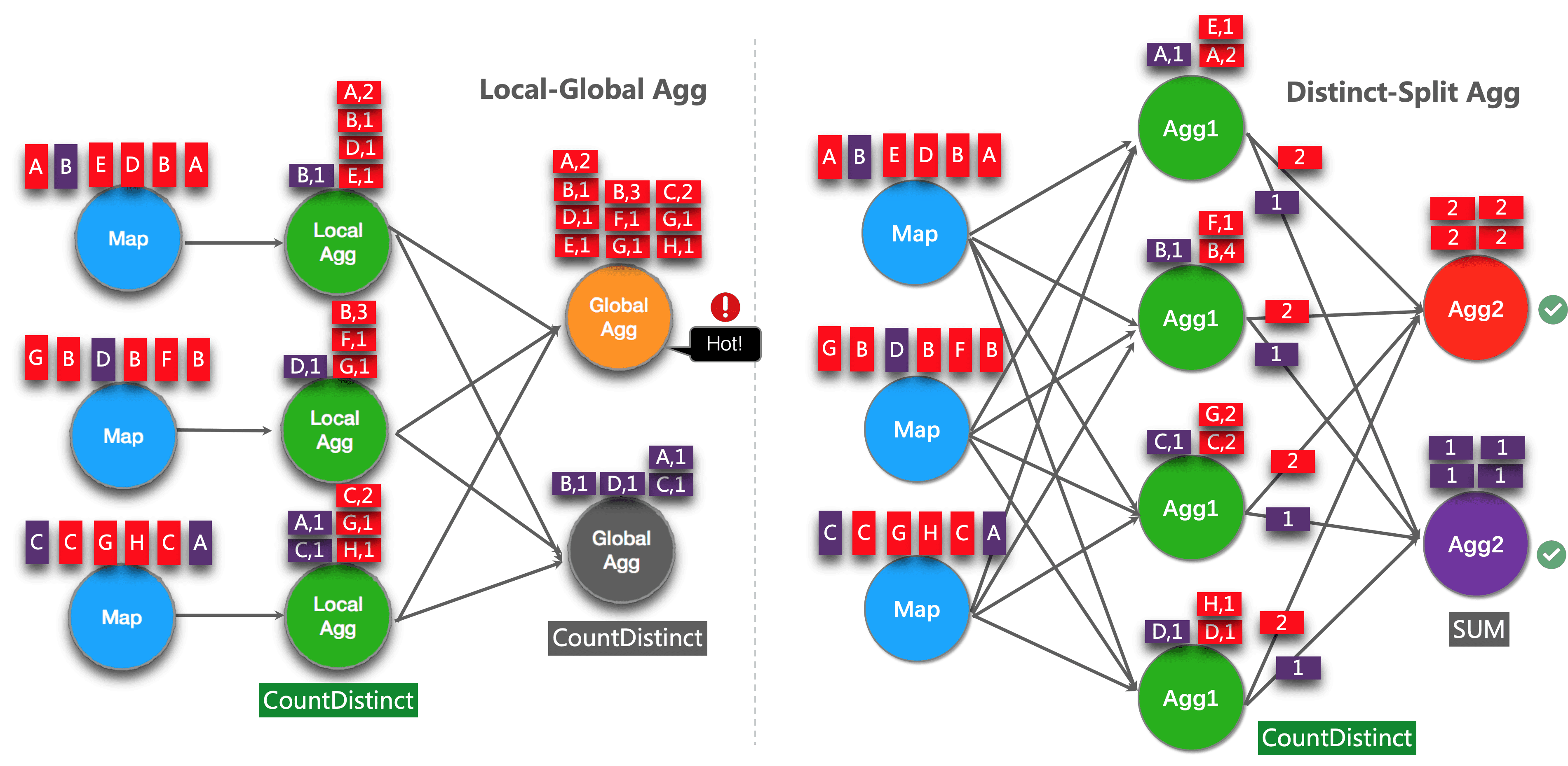
Local-Global optimization is effective to eliminate data skew for general aggregation, such as SUM, COUNT, MAX, MIN, AVG. But its performance is not satisfactory when dealing with distinct aggregation.
For example, if we want to analyse how many unique users logined today. We may have the following query:
SELECT day, COUNT(DISTINCT user_id)
FROM T
GROUP BY day
COUNT DISTINCT is not good at reducing records if the value of distinct key (i.e. user_id) is sparse. Even if local-global optimization is enabled, it doesn’t help much. Because the accumulator still contain almost all the raw records, and the global aggregation will be the bottleneck (most of the heavy accumulators are processed by one task, i.e. on the same day).
The idea of this optimization is splitting distinct aggregation (e.g. COUNT(DISTINCT col)) into two levels. The first aggregation is shuffled by group key and an additional bucket key. The bucket key is calculated using HASH_CODE(distinct_key) % BUCKET_NUM. BUCKET_NUM is 1024 by default, and can be configured by table.optimizer.distinct-agg.split.bucket-num option.
The second aggregation is shuffled by the original group key, and use SUM to aggregate COUNT DISTINCT values from different buckets. Because the same distinct key will only be calculated in the same bucket, so the transformation is equivalent.
The bucket key plays the role of an additional group key to share the burden of hotspot in group key. The bucket key makes the job to be scalability to solve data-skew/hotspot in distinct aggregations.
After split distinct aggregate, the above query will be rewritten into the following query automatically:
SELECT day, SUM(cnt)
FROM (
    SELECT day, COUNT(DISTINCT user_id) as cnt
    FROM T
    GROUP BY day, MOD(HASH_CODE(user_id), 1024)
)
GROUP BY day
The following figure shows how the split distinct aggregation improve performance (assuming color represents days, and letter represents user_id).
NOTE: Above is the simplest example which can benefit from this optimization. Besides that, Flink supports to split more complex aggregation queries, for example, more than one distinct aggregates with different distinct key (e.g. COUNT(DISTINCT a), SUM(DISTINCT b)), works with other non-distinct aggregates (e.g. SUM, MAX, MIN, COUNT).
Currently, the split optimization doesn’t support aggregations which contains user defined AggregateFunction.
The following examples show how to enable the split distinct aggregation optimization.
// instantiate table environment
TableEnvironment tEnv = ...;

tEnv.getConfig()
  .set("table.optimizer.distinct-agg.split.enabled", "true");  // enable distinct agg split
// instantiate table environment
val tEnv: TableEnvironment = ...

tEnv.getConfig
  .set("table.optimizer.distinct-agg.split.enabled", "true")  // enable distinct agg split
# instantiate table environment
t_env = ...

t_env.get_config().set("table.optimizer.distinct-agg.split.enabled", "true") # enable distinct agg split
Use FILTER Modifier on Distinct Aggregates #
In some cases, user may need to calculate the number of UV (unique visitor) from different dimensions, e.g. UV from Android, UV from iPhone, UV from Web and the total UV.
Many users will choose CASE WHEN to support this, for example:
SELECT
 day,
 COUNT(DISTINCT user_id) AS total_uv,
 COUNT(DISTINCT CASE WHEN flag IN ('android', 'iphone') THEN user_id ELSE NULL END) AS app_uv,
 COUNT(DISTINCT CASE WHEN flag IN ('wap', 'other') THEN user_id ELSE NULL END) AS web_uv
FROM T
GROUP BY day
However, it is recommended to use FILTER syntax instead of CASE WHEN in this case. Because FILTER is more compliant with the SQL standard and will get much more performance improvement.
FILTER is a modifier used on an aggregate function to limit the values used in an aggregation. Replace the above example with FILTER modifier as following:
SELECT
 day,
 COUNT(DISTINCT user_id) AS total_uv,
 COUNT(DISTINCT user_id) FILTER (WHERE flag IN ('android', 'iphone')) AS app_uv,
 COUNT(DISTINCT user_id) FILTER (WHERE flag IN ('wap', 'other')) AS web_uv
FROM T
GROUP BY day
Flink SQL optimizer can recognize the different filter arguments on the same distinct key. For example, in the above example, all the three COUNT DISTINCT are on user_id column.
Then Flink can use just one shared state instance instead of three state instances to reduce state access and state size. In some workloads, this can get significant performance improvements.
MiniBatch Regular Joins #
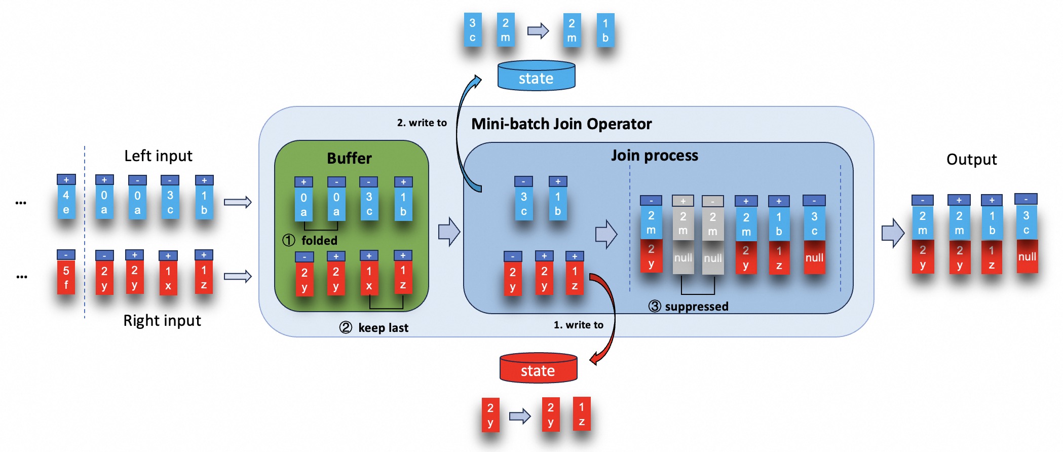
By default, regular join operator processes input records one by one, i.e., (1) lookup associated records from the state of counterpart based on the join key of the current input record, (2) update the state by adding current input record or retracting it, (3) output the join results according to the current record and associated records. This processing pattern may increase the overhead of StateBackend (especially for RocksDB StateBackend). Besides, this can lead to severe record amplification, especially in cascading join scenarios, generating too many intermediate results and further leading to performance degradation.
MiniBatch join seeks to resolve the aforementioned issues. Its core idea is to cache a bundle of inputs in a buffer inside of the mini-batch join operator.
Once the buffer reaches a specified size or time threshold, the records are forwarded to the join process.
There are two core optimizations:
- fold records in the buffer to reduce the number of data before join process.
- try best to suppress outputting redundant results when the records in buffer are being processed.
For example, consider following SQL:
SET 'table.exec.mini-batch.enabled' = 'true';
SET 'table.exec.mini-batch.allow-latency' = '5S';
SET 'table.exec.mini-batch.size' = '5000';

SELECT a.id as a_id, a.a_content, b.id as b_id, b.b_content
FROM a LEFT JOIN b
ON a.id = b.id
Both the left and right input side have unique key contained by join key which is id (assuming the number represents id, and letter represents the content).
The execution of mini-batch join operator are as shown in the figure below.
MiniBatch optimization is disabled by default for regular join. In order to enable this optimization, you should set options table.exec.mini-batch.enabled, table.exec.mini-batch.allow-latency and table.exec.mini-batch.size. Please see configuration page for more details.
Multiple Regular Joins #
StreamingStreaming Flink jobs with multiple non-temporal regular joins often experience operational instability and performance degradation due to large state sizes. This is often because the intermediate state created by a chain of joins is much larger than the input state itself. In Flink 2.1, we introduce a new multi-join operator, an optimization designed to significantly reduce state size and improve performance for join pipelines that involve record amplification and large intermediate state. This new operator eliminates the need to store intermediate state for joins across multiple tables by processing joins across various input streams simultaneously. This “zero intermediate state” approach primarily targets state reduction, offering substantial benefits in resource consumption and operational stability in some cases. This technique exchanges a reduction in storage requirements for a corresponding increase in computational effort, as intermediate states are re-evaluated upon necessity.
In most joins, a significant portion of processing time is spent fetching records from the state. The efficiency of the MultiJoin operator largely depends on the size of this intermediate state and the selectivity of the common join key(s). In a common scenario where a pipeline experiences record amplification—meaning each join produces more data and records than the previous one, the MultiJoin operator is more efficient. This is because it keeps the state on which the operator interacts much smaller, leading to a more stable operator. If a chain of joins actually produces less state than the original records, the MultiJoin operator will still use less state overall. However, in this specific case, binary joins might perform better because the state that the final joins need to operate on is smaller.
The MultiJoin Operator #
The main benefits of the MultiJoin operator are:
- Considerably smaller state size due to zero intermediate state.
- Improved performance for chained joins with record amplification.
- Improved stability: linear state growth with amount of records processed, instead of polynomial growth with binary joins.
Also, pipelines with MultiJoin instead of binary joins usually have faster initialization and recovery times due to smaller state and fewer nodes.
When to enable the MultiJoin? #
If your job has multiple joins that share at least one common join key, and you observe that the intermediate state in the intermediate joins is larger than the input sources, consider enabling the MultiJoin operator.
Recommended use cases:
- The common join key(s) have a high selectivity (the number of records per key is small)
- Statement with several chained joins and considerable intermediate state
- No considerable data skew on the common join key(s)
- Joins are generating large state (state 50+ GB)
If your common join key(s) exhibit low selectivity (i.e., a high number of rows sharing the same key value), the MultiJoin operator’s required recomputation of the intermediate state can severely impact performance. In such scenarios, binary joins are recommended, as these will partition the data using all join keys.
How to enable the MultiJoin? #
To enable this optimization globally for all eligible joins, set the following configuration:
SET 'table.optimizer.multi-join.enabled' = 'true';
Alternatively, you can enable the MultiJoin operator for specific tables using the MULTI_JOIN hint:
SELECT /*+ MULTI_JOIN(t1, t2, t3) */ * FROM t1
JOIN t2 ON t1.id = t2.id
JOIN t3 ON t1.id = t3.id;
The hint approach allows you to selectively apply the MultiJoin optimization to specific query blocks without enabling it globally. For more details on the MULTI_JOIN hint, see Join Hints. The configuration setting takes precedence over the hint.
Important: This is currently in an experimental state - optimizations and breaking changes might be implemented. We currently support only streaming INNER/LEFT joins. Due to records partitioning, you need at least one key that is shared between the join conditions, see:
- Supported: A JOIN B ON A.key = B.key JOIN C ON A.key = C.key (Partition by key)
- Supported: A JOIN B ON A.key = B.key JOIN C ON B.key = C.key (Partition by key via transitivity)
- Not supported: A JOIN B ON A.key1 = B.key1 JOIN C ON B.key2 = C.key2 (No single key allows partitioning A, B, and C together in a single operator. This will be split into multiple MultiJoin operators)
MultiJoin Operator Example - Benchmark #
Here’s a 10-way benchmark between the default binary joins and the MultiJoin operator. You can observe the amount of intermediate state in the first section, the amount of records processed when the operators reach 100% busyness in the second section, and the checkpoints in the third.
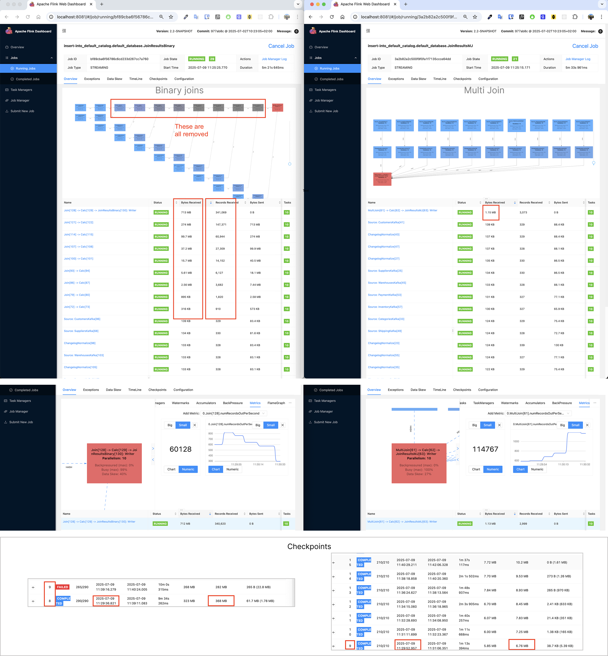
For this 10-way join above, involving record amplification, we’ve observed significant improvements. Here are some rough numbers:
- Performance: 2x to over 100x+ increase in processed records when both at 100% busyness.
- State Size: 3x to over 1000x+ smaller as intermediate state grows.
The total state is always smaller with the MultiJoin operator. In this case, the performance is initially the same, but as the intermediate state grows, the performance of binary joins degrades and the multi join remains stable and outperforms.
This general benchmark for the 10-way join was run with the following configuration: 1 record per tenant_id (high selectivity), 10 upsert kafka topics, 10 parallelism, 1 record per second per topic. We used rocksdb with unaligned checkpoints and with incremental checkpoints. Each job ran in one TaskManager containing 8GB process memory, 1GB off-heap memory and 20% network memory. The JobManager had 4GB process memory. The host machine contained a M1 processor chip, 32GB RAM and 1TB SSD. The sink uses a blackhole connector so we only benchmark the joins. The SQL used to generate the benchmark data had this structure:
INSERT INTO JoinResultsMJ
SELECT *all fields*
FROM TenantKafka t
         LEFT JOIN SuppliersKafka s ON t.tenant_id = s.tenant_id AND ...
         LEFT JOIN ProductsKafka p ON t.tenant_id = p.tenant_id AND ...
         LEFT JOIN CategoriesKafka c ON t.tenant_id = c.tenant_id AND ...
         LEFT JOIN OrdersKafka o ON t.tenant_id = o.tenant_id AND ...
         LEFT JOIN CustomersKafka cust ON t.tenant_id = cust.tenant_id AND ...
         LEFT JOIN WarehousesKafka w ON t.tenant_id = w.tenant_id AND ...
         LEFT JOIN ShippingKafka sh ON t.tenant_id = sh.tenant_id AND ...
         LEFT JOIN PaymentKafka pay ON t.tenant_id = pay.tenant_id AND ...
         LEFT JOIN InventoryKafka i ON t.tenant_id = i.tenant_id AND ...;
Delta Joins #
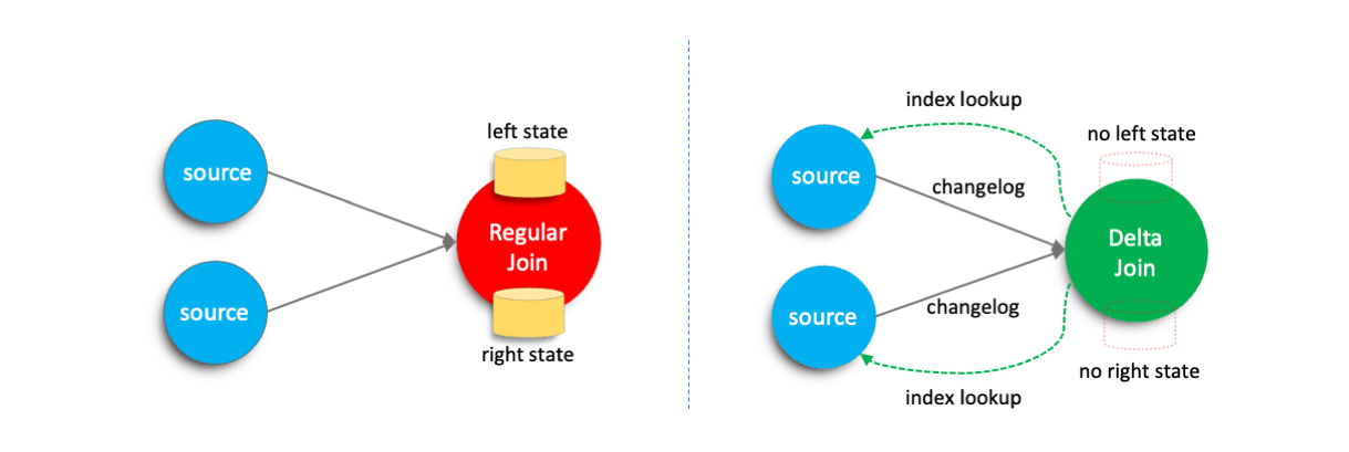
In streaming jobs, regular joins keep all historical data from both inputs to ensure accuracy. Over time, this causes the state to grow continuously, increasing resource usage and impacting stability.
To mitigate these challenges, Flink introduces the delta join operator. The key idea is to replace the large state maintained by regular joins with a bidirectional lookup-based join that directly reuses data from the source tables. Compared to traditional regular joins, delta joins substantially reduce state size, enhances job stability, and lowers overall resource consumption.
This feature is enabled by default. A regular join will be automatically optimized into a delta join when all the following conditions are met:
- The sql pattern satisfies the optimization criteria. For details, please refer to Supported Features and Limitations
- The external storage system of the source table provides index information for fast querying for delta joins. Currently, Apache Fluss(Incubating) has provided index information at the table level for Flink, allowing such tables to be used as source tables for delta joins. Please refer to the Fluss documentation for more details.
Working Principle #
In Flink, regular joins store all incoming records from both input sides in the state to ensure that corresponding records can be matched correctly when data arrives from the opposite side.
In contrast, delta joins leverage the indexing capabilities of external storage systems. Instead of performing state lookups, delta joins issue efficient index-based queries directly against the external storage to retrieve matching records. This approach eliminates redundant data storage between the Flink state and the external system.
Important Configurations #
Delta join optimization is enabled by default. You can disable this feature manually by setting the following configuration:
SET 'table.optimizer.delta-join.strategy' = 'NONE';
Please see Configuration page for more details.
To fine-tune the performance of delta joins, you can also configure the following parameters:
table.exec.delta-join.cache-enabledtable.exec.delta-join.left.cache-sizetable.exec.delta-join.right.cache-size
Please see Configuration page for more details.
Supported Features and Limitations #
Delta joins are continuously evolving, and supports the following features currently.
- Support for INSERT-only tables as source tables.
- Support for CDC tables without DELETE operations as source tables.
- Support for projection and filter operations between the source and the delta join.
- Support for caching within the delta join operator.
However, Delta Joins also have several limitations. Jobs containing any of the following conditions cannot be optimized into a delta join:
- The index key of the table must be included in the join’s equivalence conditions.
- Only INNER JOIN is currently supported.
- The downstream operator must be able to handle duplicate changes, such as a sink operating in UPSERT mode without
upsertMaterialize. - When consuming a CDC stream, the join key must be part of the primary key.
- When consuming a CDC stream, all filters must be applied on the upsert key.
- Non-deterministic functions are not allowed in filters or projections.